Computing Eigenstates

In this section we show how to compute eigenstates on the example of the Henon-Heiles potential. This two-dimensional potential in the variables and is given by:

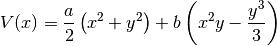
where we set and . To compute the eigenstates we write a configuration file eigenstates.py like:

dimension = 2
ncomponents = 1

potential = "henon_heiles"

eigenstate_of_level = 0

eigenstates_indices = [0, 1, 2, 3, 4, 5, 6, 7, 8, 9, 10, 11, 12, 13, 14]

starting_point = [0.5, 0.5]

eps = 0.25

hawp_template = {
    "type": "HagedornWavepacket",
    "dimension": dimension,
    "ncomponents": 1,
    "eps": eps,
    "basis_shapes": [{
        "type": "HyperbolicCutShape",
        "K": 24,
        "dimension": dimension
    }]
}

innerproduct = {
    "type": "HomogeneousInnerProduct",
    "delegate": {
        "type": "DirectHomogeneousQuadrature",
        'qr': {
            'type': 'TensorProductQR',
            'dimension': dimension,
            'qr_rules': [{'dimension': 1, 'order': 32, 'type': 'GaussHermiteQR'},
                         {'dimension': 1, 'order': 32, 'type': 'GaussHermiteQR'}]
        }
    }
}

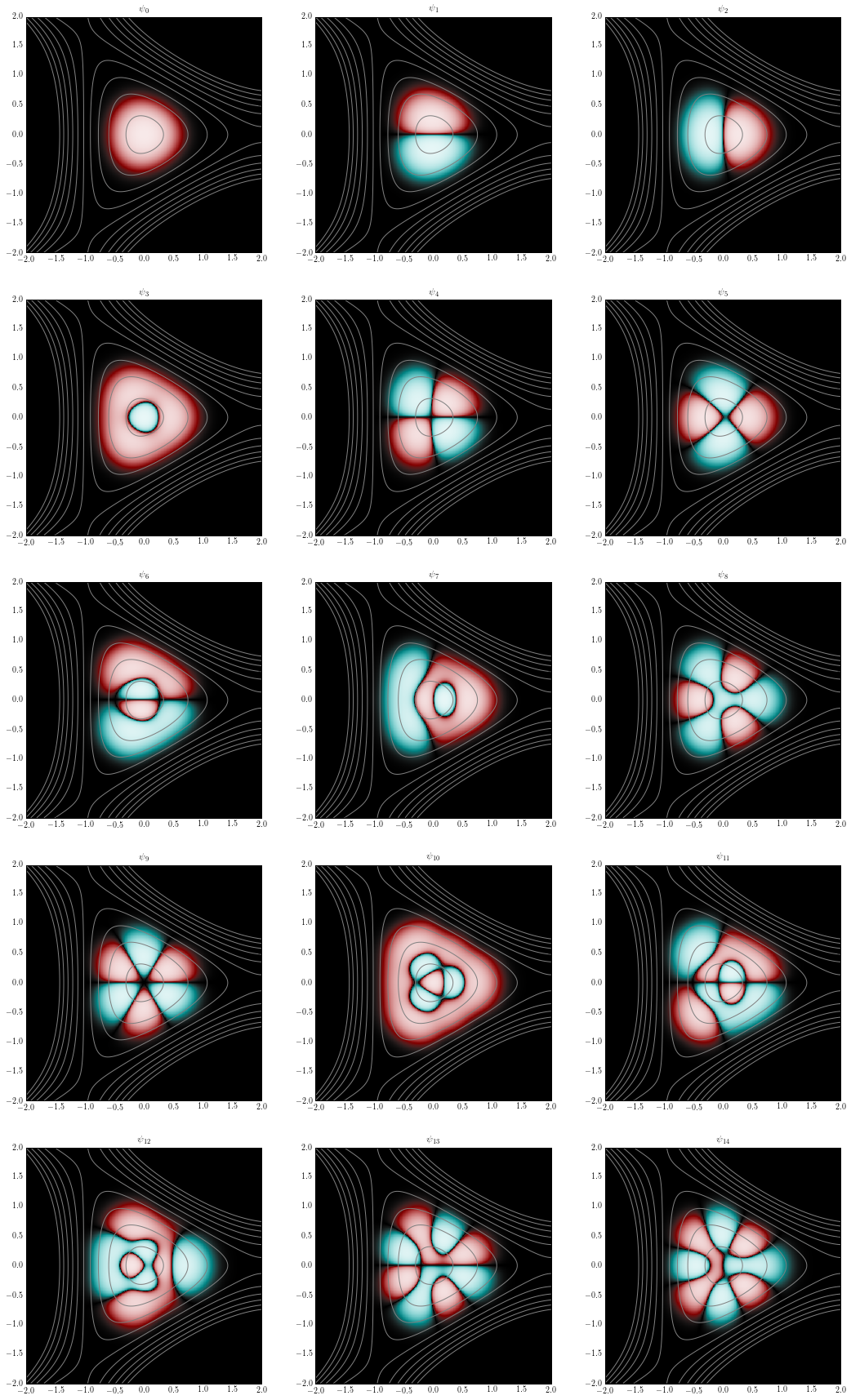
We compute the first 15 eigenstates up to . The parameter starting_point sets the starting value for the minimization of the potential surface. This value is choosen such to stay in the local minimum we are interested in. The basis consists of the space spanned by all wavepackets indexed in the hyperbolic cut having sparsity . The actual computation is done by using the script ComputeEigenstates.py:

ComputeEigenstates.py eigenstates.py

and will print some output:

Using configuration from file: eigenstates.py
Requested function: add_parameters
Plugin to load: IOM_plugin_parameters
Optimization terminated successfully.
         Current function value: 0.000000
         Iterations: 98
         Function evaluations: 189
----------------------------------------------------------------------
Parameter values are:
---------------------
 q0:
[[  2.24608505e-13]
 [  3.33457394e-13]]
 p0:
[[ 0.]
 [ 0.]]
 Q0:
[[  1.00000000e+00+0.j  -5.62327962e-14-0.j]
 [ -5.62883073e-14+0.j   1.00000000e+00+0.j]]
 P0:
[[ 0. +1.00000000e+00j  0. +5.62327962e-14j]
 [ 0. +5.62883073e-14j  0. +1.00000000e+00j]]
 Consistency check:
   P^T Q - Q^T P  =?=  0
[[ 0. +0.00000000e+00j  0. +1.11022302e-16j]
 [ 0. -1.11022302e-16j  0. +0.00000000e+00j]]
   Q^H P - P^H Q  =?=  2i
[[ 0. +2.00000000e+00j  0. +1.26217745e-29j]
 [ 0. +1.26217745e-29j  0. +2.00000000e+00j]]
Warning: no inner product specified!
----------------------------------------------------------------------
State: 0
Energy: 0.0623898880123
Coefficients:

[  9.99697146e-01+0.j   7.06667357e-09+0.j   1.88119658e-03+0.j
   1.22024364e-02+0.j   8.31557109e-04+0.j   1.61933847e-04+0.j
   3.51763774e-04+0.j   6.28914248e-05+0.j   1.48819058e-05+0.j
   1.53830363e-05+0.j   4.64872426e-06+0.j   1.40044195e-06+0.j
   9.48658758e-07+0.j   3.83630231e-07+0.j   1.42241989e-07+0.j
   7.84302527e-08+0.j   3.66375058e-08+0.j   1.58225631e-08+0.j
...

and produce an eigenstates.hdf5 file containing all the wavepackets computed. Next we compute norms and energies of these states by:

ComputeNorms.py -d eigenstates.hdf5
ComputeEnergies.py -d eigenstates.hdf5

We could also evaluate and plot the packets or call any other post-processing script. But we like to do some custom computations and therefore switch to an interactive Python session now:

BF = BlockFactory()
IOM = IOManager()

IOM.open_file("eigenstates.hdf5")
PA = IOM.load_parameters()

V = BF.create_potential(PA)

Load the wavepackets:

packets = [IOM.load_wavepacket(0, blockid=i) for i in xrange(15)]

Set up a grid for evaluation:

x = linspace(-2, 2, 500)
y = linspace(-2, 2, 500)
X, Y = meshgrid(x, y)
M = row_stack([X.reshape(1,-1), Y.reshape(1,-1)])

and evaluate potential as well as eigenstates on this grid:

v = V.evaluate_at(M, entry=(0,0)).reshape(500,500).T

psis = [hawp.evaluate_at(M, prefactor=True, component=0).reshape(500,500) for hawp in packets]

Plot the eigenstates together with the potential contour lines:

figure(figsize=(18,30))

for i, psi in enumerate(psis):

    subplot(5, 3, i+1)
    plotcf2d(x, y, psi, darken=0.1)
    contour(x, y, v, linspace(0.05, 1.5, 10), colors="gray")
    title(r"$\psi_{%d}$" % i)

savefig("henon_heiles_eigenstates.png")

We check that the eigenstates are properly normalized:

N = [IOM.load_norm(blockid=i) for i in xrange(15)]
N

[array([[ 1.]]),
 array([[ 1.]]),
 array([[ 1.]]),
 array([[ 1.]]),
 array([[ 1.]]),
 array([[ 1.]]),
 array([[ 1.]]),
 array([[ 1.]]),
 array([[ 1.]]),
 array([[ 1.]]),
 array([[ 1.]]),
 array([[ 1.]]),
 array([[ 1.]]),
 array([[ 1.]]),
 array([[ 1.]])]

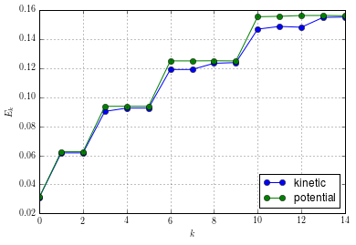
Finally, look at the energies of these states:

E = squeeze(array([IOM.load_energy(blockid=i) for i in xrange(15)]))

array([[ 0.03113906,  0.03125083],
       [ 0.06171018,  0.06251042],
       [ 0.06171017,  0.06251044],
       [ 0.09028264,  0.09378443],
       [ 0.09254484,  0.09379187],
       [ 0.09254101,  0.0937974 ],
       [ 0.11912411,  0.12505747],
       [ 0.11914656,  0.12503636],
       [ 0.12341898,  0.12514402],
       [ 0.12387966,  0.12501247],
       [ 0.14693627,  0.15548814],
       [ 0.14879932,  0.15576321],
       [ 0.14824844,  0.15631414],
       [ 0.15502718,  0.156359  ],
       [ 0.15527243,  0.15615653]])

and then plot the energy levels:

figure()
plot(arange(15), E[:,0], "-o", label=r"kinetic")
plot(arange(15), E[:,1], "-o", label=r"potential")
grid(True)
legend(loc="lower right")
xlabel(r"$k$")
ylabel(r"$E_k$")

We can also easily compute the total energy:

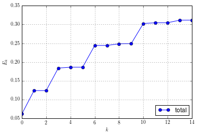
Etot = sum(E, axis=1)

array([ 0.06238989,  0.12422061,  0.12422061,  0.18406707,  0.18633672,
        0.18633841,  0.24418158,  0.24418292,  0.248563  ,  0.24889214,
        0.3024244 ,  0.30456252,  0.30456258,  0.31138619,  0.31142895])

and again plot the energy levels based on these data:

figure()
plot(arange(15), Etot, "-o", label=r"total")
grid(True)
xlabel(r"$k$")
ylabel(r"$E_k$")
legend(loc="lower right")